CIS 1051 - Temple Rome Spring 2023

Intro to Problem solving and

Programming in Python

Functions and return values

Prof. Andrea Gallegati

( tuj81353@temple.edu )

Return Values

Many of Python intrinsic functions (e.g. math functions, here below) return values, but the functions we’ve written so far are all void:

they have an effect, like printing a value or moving a turtle, but they don’t have a return value. More precisely, their return value is None.

import math

e = math.exp(1.0)

radius = 2.0 ; radians = 3.14
height = radius * math.sin(radians)

Contrary, return values are usually assigned to a variable or used as part of an expression.

A first example can be area, which returns the area of a circle given its radius.

def area(radius):
    a = math.pi * radius**2
    return a

We have already seen the return statement before, but here it includes an expression.

It means: “Return immediately from this function and use the following expression as a return value.”

The expression can be arbitrarily complicated, e.g. the above function becomes more concisely:

def area(radius):
    return math.pi * radius**2

On the other hand, temporary variables make debugging easier.

It is possible to have multiple return statements, e.g. one in each branch of a conditional:

def absolute_value(x):
    if x < 0:
        return -x
    else:
        return x

Since they are in an alternative conditional, just one runs!

As a return statement runs, the function terminates without executing any subsequent statements: the code after a return statement is called dead code. The same for any other place the flow of execution can never reach.

Always ensure that every possible path through a program hits a return statement!

def absolute_value(x):
    if x < 0:
        return -x
    if x > 0:
        return x

This is incorrect since when x is 0, neither condition is true, and the function ends without hitting a return statement.

Thus, the return value is None, which is not the absolute value of 0 !

abs = absolute_value(0)
print(abs)

None

By the way, Python provides a built-in function called abs that computes absolute values.

Incremental Development

Writing larger functions usually means spending more time debugging.

To deal with increasingly complex programs, try out a process called incremental development.

The goal: avoid long debugging sessions by adding and testing only a small amount of code at a time.

If we want to find the distance between two points, given by their coordinates $(x_1,\: y_1)$ and $(x_2,\: y_2)$, by the Pythagorean theorem their distance is:

$$ \text{d} = \sqrt{(\: x_2 - \: x_1 \:)^2 + (\: y_2 - \: y_1 \:)^2} $$

First step is to consider what a distance function should look like in Python:

• what are the inputs? (parameters)
• what is the output? (return value)

Here:

• inputs are two points, we can represent using four numbers
• return value is the distance, a floating-point value

We can thus write immediately an outline of that function:

def distance(x1, y1, x2, y2):
    return 0.0

Obviously, this version doesn’t work ... or better, it doesn't compute distances; it always returns zero.

But it is syntactically correct, and it runs, thus we can test it before making it more complicated.

Let's test the new function, calling it with sample arguments:

d = distance(1, 2, 4, 6)
print(d)

0.0

The chosen values are such that the distance (5) is the hypotenuse of a right triangle.

When testing a function, it is useful to know the right answer!

Confirmed that – so far – the function is syntactically correct, we can start adding code to the body.

As a next step, it is reasonable to find the differences $(\: x_2 - \: x_1 \:)$ and $(\: y_2 - \: y_1 \:)$.

def distance(x1, y1, x2, y2):
    dx = x2 - x1
    dy = y2 - y1
    print('dx is', dx)
    print('dy is', dy)
    return 0.0

This version stores those values in temporary variables and prints them:

d = distance(1, 2, 4, 6)

dx is 3
dy is 4

If the function is working, we know that:

• it is getting the right arguments
• it is performing the first computation correctly.

If not, there are only a few lines to check.

Next we compute the sum of squares of dx and dy:

def distance(x1, y1, x2, y2):
    dx = x2 - x1
    dy = y2 - y1
    dsquared = dx**2 + dy**2
    print('dsquared is: ', dsquared)
    return 0.0

Again, run the program to check the output.

d = distance(1, 2, 4, 6)

dsquared is:  25

Finally, use math.sqrt to compute and return the result:

def distance(x1, y1, x2, y2):
    dx = x2 - x1
    dy = y2 - y1
    dsquared = dx**2 + dy**2
    result = math.sqrt(dsquared)
    return result

If that works correctly, you are done, if not print the result value before the return statement.

d = distance(1, 2, 4, 6)

This final version doesn’t display anything; it only returns a value.

Print statements are useful for debugging, but once we get the function working, we should remove them.

Code like this (aka scaffolding) is helpful for building the program, but is never part of the final product!

With more experience, we might write and debug bigger chunks, but incremental development always saves a lot of debugging time.

Composition

We can call one function from within another.

For example, we will write a function that:

• takes two points
  • a circle center, stored in xc and yc
  • a point on the perimeter, in xp and yp
• computes the area of that circle

xc = 1; yc = 2
xp = 4; yp = 6

First step is to find the radius, i.e. the distance between the two points.

We just wrote a function, distance, that does that:

radius = distance(xc, yc, xp, yp)

Next step is to find the area of a circle with that radius.

We just wrote that too:

result = area(radius)

Just encapsulate these two within a function

def circle_area(xc, yc, xp, yp):
    radius = distance(xc, yc, xp, yp)
    result = area(radius)
    return result

and get rid of temporary variables (useful to dev/debug), once working, to make it more concise:

def circle_area(xc, yc, xp, yp):
    return area(distance(xc, yc, xp, yp))

Boolean functions

Functions can return booleans.

It is convenient to hide complicated tests inside functions.

def is_divisible(x, y):
    if x % y == 0:
        return True
    else:
        return False

It is common to give boolean functions names that sound like yes/no questions.

is_divisible(6, 4)

False

is_divisible(6, 3)

True

The == operator returns a boolean, thus we can rewrite the above function more concisely

def is_divisible(x, y):
    return x % y == 0

Boolean functions are often used in conditional statements:

x = 6 ; y = 3
if is_divisible(x, y):
    print('x is divisible by y')

x is divisible by y

It might be tempting to write something like

if is_divisible(x, y) == True:
    print('x is divisible by y')

x is divisible by y

... but the extra comparison is unnecessary.

More Recursion

Although just a small subset of Python has been covered, so far, we got convinced that anything that can be computed can be expressed in this language.

In other words, this subset is a complete programming language by itself.

Any program ever written could be rewritten using only the language features we have learned so far (maybe with a few more commands to control devices like the mouse, keyboard, etc., but that’s all – the same as for the pygame module).

Proving that claim (Turing Thesis) is a nontrivial exercise first accomplished by Alan Turing, a mathematician and one of the first computer scientists!

As recommended by your book, have a look at Michael Sipser’s "Introduction to the Theory of Computation (Course Technology, 2012)".

To get a better idea of what we can do with what we learned so far, let's evaluate a few recursively defined mathematical functions.

A recursive definition contains a reference to the thing being defined, e.g. the factorial function!

$$ \begin{cases} 0! = 1 \\ n! = n(n-1)! \end{cases} $$

A truly circular definition is not that useful: vorpal: An adjective used to describe something that is vorpal.

If we can write a recursive definition of something, we can write a Python program to evaluate it!

First, decide what the parameters should be: it clearly takes an integer.

def factorial(n):
    if n == 0:
        return 1

Then, if the argument is 0 return 1.

Otherwise, make a recursive call to the factorial of n-1 and multiply it by n:

def factorial(n):
    if n == 0:
        return 1
    else:
        recurse = factorial(n-1)
        result = n * recurse
        return result

The flow of execution is similar to the countdown function, if evaluating the 3!

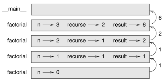
The return values are being passed back up the stack, being the product of n and recurse.

Leap of Faith

Following the flow of execution is one way to read programs, but it quickly becomes overwhelming.

An alternative is what your book calls the “leap of faith”:

... instead of following the flow of execution, assume that the function works correctly and returns the right result.

This is what we did so far, when using built-in functions: we don’t examine these functions bodies, but just assume they were written by good programmers and simply works!

The same is true when calling one of your own functions: once convinced it is correct – by examining the code and testing – just use it without looking at the body again.

Again, the same is true of recursive programs: instead of following the flow of execution, assume that the recursive call works (aka returns correct results) before using it, writing a recursive procedure!

For example:

“ Assuming I can find the factorial of n-1, can I compute the factorial of n?

Yes, simply multiplying it by n! "

Of course, it’s a bit strange ... that’s why it’s called a leap of faith!

Even more Recursion

Another example of a recursively defined mathematical function is Fibonacci sequence

$$ \begin{cases} F_0 = 0 \\ F_1 = 1 \\ F_n = F_{n-1} + F_{n-2} \end{cases} $$

https://en.wikipedia.org/wiki/Fibonacci_number

... that in Python looks like this

def fibonacci (n):
    if n == 0:
        return 0
    elif  n == 1:
        return 1
    else:
        return fibonacci(n-1) + fibonacci(n-2)

Trying to follow the flow of execution here, will make your head explode.

Thus, according to the leap of faith: assume the two recursive calls work correctly.

It is clear you get the right result by adding them together!

Checking Types

What happens if we call factorial and give it 1.5 as an argument?

factorial(1.5)

---------------------------------------------------------------------------
RuntimeError                              Traceback (most recent call last)
<ipython-input-58-e28385ff5339> in <module>()
----> 1 factorial(1.5)

<ipython-input-56-e2257ac15153> in factorial(n)
      3         return 1
      4     else:
----> 5         recurse = factorial(n-1)
      6         result = n * recurse
      7         return result

... last 1 frames repeated, from the frame below ...

<ipython-input-56-e2257ac15153> in factorial(n)
      3         return 1
      4     else:
----> 5         recurse = factorial(n-1)
      6         result = n * recurse
      7         return result

RuntimeError: maximum recursion depth exceeded in comparison

This is an infinite recursion.

Weird!

The function has a base case when n == 0.

If n is not an integer, we can miss the base case and recurse forever...

• In the first recursive call, the value of n is 0.5.
• In the next, it is -0.5.
• Then, it gets smaller (more negative) and never reaches 0.

We have two choices.

• try to generalize the factorial (floating-point).
• make factorial check the type of its argument (integer).

First option is the gamma function: a little beyond the scope of this class.

We’ll go for the second.

Use the built-in function isinstance to verify the type of the argument and then make sure it is positive:

def factorial (n):
    if not isinstance(n, int):
        print('Factorial is only defined for integers.')
        return None
    elif n < 0:
        print('Factorial is not defined for negative integers.')
        return None
    elif n == 0:
        return 1
    else:
        return n * factorial(n-1)

In the first two cases, it prints an error message and returns None (indicating something went wrong)

factorial('fred')

Factorial is only defined for integers.

factorial(-2)

Factorial is not defined for negative integers.

If we get past both checks, we know that n is positive or zero, being sure the recursion terminates.

This Design Pattern is called a guardian: protecting the code from values that might cause an error.

Moreover, we will soon introduce a more flexible alternative to printing an error message: raising an exception.

Debugging

Breaking a large program into smaller functions creates natural checkpoints for debugging.

If a function is not working, there is something wrong with the:

• arguments, violated precondition.
• function, violated postcondition.
• return value or the way it is being used.

• First, add a print at the function beginning to display the parameters' values/types.
• Second, add a print before each return statement to display the return value.
• Last, look at the function call to make sure the return value is being used correctly.

Adding print statements at the function beginning/end helps visualizing the flow of execution. For example:

def factorial(n):
    space = ' ' * (4 * n)
    print(space, 'factorial', n)
    if n == 0:
        print(space, 'returning 1')
        return 1
    else:
        recurse = factorial(n-1)
        result = n * recurse
        print(space, 'returning', result)
        return result

space is a string of space characters that controls the indentation of the output

factorial(4)

                 factorial 4
             factorial 3
         factorial 2
     factorial 1
 factorial 0
 returning 1
     returning 1
         returning 2
             returning 6
                 returning 24

24

It takes some time to develop even a little of effective scaffolding, but it saves a lot of debugging.